ESE315 Assignment 2
From atmoschem
Required:
- (20 credits) Mars is 2.3e8 km away from the Sun; its albedo is 0.15. Its only source of heat is solar radiation. (a) Calculate the effective temperature of Mars. (b) The temperature observed at the surface of Mars is 220 K. What do you conclude about the Martian atmosphere?
- (20 credits) The Earth's effective temperature during distant past may be much lower than the current value. This is because the Sun's radiation during its early years may be 30% weaker than what it is now. Assuming that the distance between the Sun and the Earth has not changed significantly since the time of the Earth's formation 4.6 billion years ago. Use python to make a 2-D contour plot of the Earth's effective temperature (Te) for a range of solar constants and a range of albedos. See this example to learn how to make 2D contour plots in python.
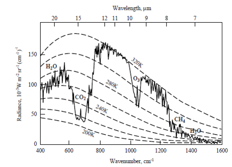
- Use the MODTRAN model to simulate the terrestrial infrared radiation spectrum at a location on Earth. Use the default present-day conditions: CO2=400 ppm; CH4=1.7 ppm; tropospheric ozone=28 ppb; stratospheric ozone scale=1; water vapor scale=1; freon scale=1; temperature offset=0C; no clouds or rain; altitude 70 km; looking down. Choose a location and clearly indicate it.
- (20 credits) Plot the total radiance as a function of wavelength in micrometers. Be careful of the units! (Tips: there are many ways to read data into python. We recommend that you download the data, delete the irrelevant part, and then use the 'pandas' package to import data. See tutorials here, here, and here. )
- (20 credits) Using the Planck function, plot the blackbody radiation spectra at several different temperatures, such that the Planck function lines encompass the simulated spectra you showed in the previous question. Discuss why some of the features in your simulated spectra look like the Planck function at specific temperature (we talked about this in class). An example of the Planck function is on our Jupyter notebook server (public/planck_func_fitting.ipynb). Your result should look something like this (but with wavelengths as the x-variable):

- (20 credits) Increase the concentration of one of the greenhouse gases. Plot both the old and the new simulated spectra in one plot. Calculate and plot the difference between the two spectra. Discuss how they are related to the changes you made to the greenhouse gases.
Extra credit:
The following questions are not part of the assignment that you are required to hand in. You can do any ONE (but only ONE) of them to get 10 extra credits. Or, you can use these as inspiration for your term project.
Based on the MODTRAN model:
- Demonstrate the Band Saturation Effect by making a plot of Iout as a function of a greenhouse gas concentration, from say 0 to 1000 ppm, with lots of points at low concentrations. Explain this phenomenon.
- Calculate the average temperature that the Earth radiates to space by setting the model Iout to epsilon sigma T^4 and solving for T. What altitude is this (assuming the light is coming from the troposphere, the lowermost region in the temperature profile plot)? How does this altitude change as you change the greenhouse gas concentration? Explain this phenomenon.
- What is the effect of clouds on the upwelling IR to space, and to the downwelling IR seen from the ground? Explain this phenomenon.
- Compare CO2 vs. methane as greenhouse gases. Which would be the stronger if they had the same concentrations? Which is stronger given their current concentrations? Explain this phenomenon.
- Simulate the temperature response to greenhouse gas IR forcing by adjusting the ground temperature to maintain a constant Iout as you increase the gas concentration. Demonstrate the water vapor feedback effect by doing this using both options of constant vapor pressure and constant relative humidity. Explain this phenomenon.
- This page was last modified on 28 September 2020, at 09:05.
- This page has been accessed 12,643 times.